


Upsampling with Machine Learning

Table of Contents
Why Image Upsampling?⌗
I’ve been excited about image upsampling for over a year now, seeing it as a promising way to improve on existing video codecs. Video is the most bandwidth-intensive data format, accounting for over half of all Internet traffic. All of the new video formats like AV1 do not incorporate new advances in machine learning, so there is some possibility for independent creators like myself to produce something new and useful.
One inspirational work is LCEVC ( https://ieeexplore.ieee.org/document/9795094 ), which uses a series of upsampling steps to improve the quality of existing video codecs. Since LCEVC does not use any machine learning, I believe that it is possible to improve on it by using machine learning to do the upsampling instead. These same sorts of models can also clean up video codec artifacts, such as blockiness while restoring the original quality.
Probably the most advanced research I could find in this direction is this paper: “Dual-layer Image Compression via Adaptive Downsampling and Spatially Varying Upconversion” (Xi Zhang) https://arxiv.org/pdf/2302.06096.pdf It is the first paper that proposes transmitting both traditional compressed video and quantized encoded values from a downsampling network, which aid to improve the quality of the upsampling network. This is pretty similar to LCEVC in how it works, but it leverages machine learning instead of traditional image processing.
But, since I’m a newbie when it comes to machine learning I have to start somewhere less exciting.
Inspired by the author of Tortoise-TTS who built his own machine learning super-computer ( https://nonint.com/2022/05/30/my-deep-learning-rig/ ) and trained the world’s best open-source text-to-speech model, I’ve been working on building my own image upsampling models at home using my own hardware as a hobby project.
In the machine learning literature, these are called super-resolution models. Since they are well-studied, there are many open-source implementations available. I’ve been using the VapSR model ( https://github.com/zhoumumu/VapSR ) so far, since it is unusually small and fast for the excellent quality of its results.
Example⌗
Top-Left: Original Image. Top-Right: My model output.
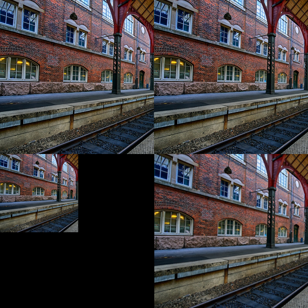
Bottom-Left: Input Image. Bottom-Right: Baseline Bicubic upsampler.
My model output is significantly better than the bicubic upsampler, such as the one used in the LCEVC codec, so imagine if we could get these sorts of results in a video codec!
The code for my project is here: https://github.com/catid/upsampling
I’ve released code to get this model to run on Intel GPUs using OpenVINO, which turns out to be about twice as fast as the CPU itself and avoids using CPU resources. If we can get these sorts of models running efficiently on Intel/AMD laptops and Android/iOS cellphones, then devices that are consuming video will be able to use these sorts of models to improve the quality of video codecs or reduce the bandwidth of video over networks.
At this point I have reached a good first milestone where I was able to train a VapSR model on my own hardware and then deploy it to run with OpenVINO. So, I’m going to share my experience here to help others who are interested in doing the same.
Hardware⌗
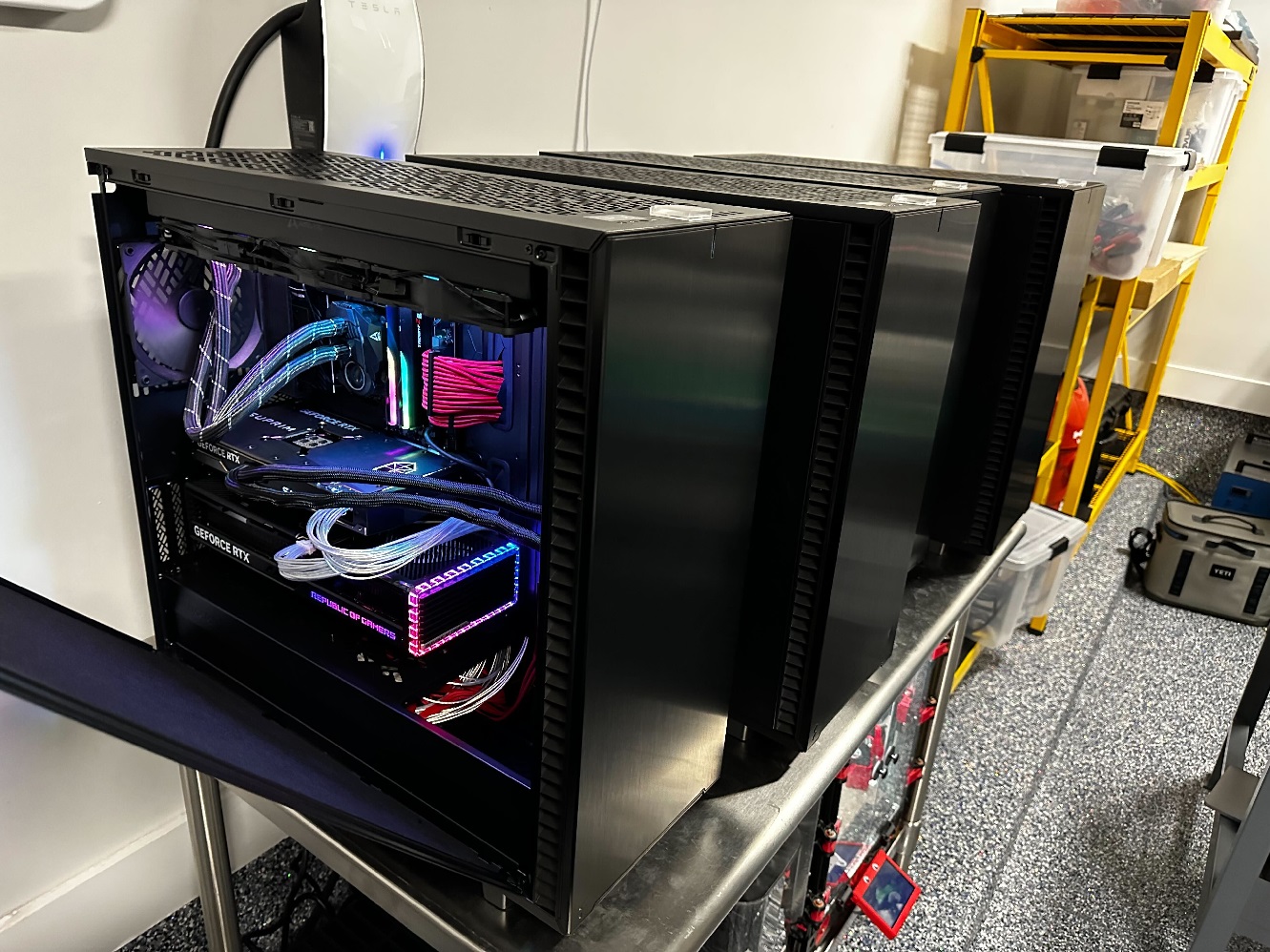
I decided to build my own machine learning training super computer cluster at home. I’ve noticed that people tend to prefer self-hosting over cloud services for training super-resolution models based on the papers I’ve been reading. So the only question was how much to spend on hardware and what type of computer to build. Since the models are small, training scales well with a cluster of computers - Each computer handles a part of the dataset and they run mostly in parallel.
Most people use 1-2 RTX 3090 cards to train their models, so my cluster of 8x RTX 4090 cards makes training pleasantly fast. Pretty much all the full training runs I’ve done have completed within 2-8 hours, which has allowed me to iterate quickly and learn faster. It’s definitely over-kill, but I’ve ended up spending a lot of time using these machines every day for the past two months, and I expect I’ll continue finding uses for them for the next few years.
There are three references that pushed me in the direction of using RTX 4090 GPUs for training.
- Lambda Labs reports that RTX 4090 has the best performance/$: https://lambdalabs.com/blog/nvidia-rtx-4090-vs-rtx-3090-deep-learning-benchmark
- Tim Dettmers has a lengthy article showing that the RTX 4090 is second only to the H100 for training performance: https://timdettmers.com/2023/01/30/which-gpu-for-deep-learning/
- Also mentioned in the Tortois-TTS blog “A lesser-known fact about 3090s is they actually pull burst currents of up to 600W.” I’ve seen this myself from previous system builds.
Note that these references mostly consider FP16 training, which I found works almost as well as FP32 training for super-resolution model training (within 0.01 dB PSNR), but trains 33% faster. Also note that RTX 4090 cards do not have NVLink, but this is not needed for anything I’m interested in doing.
I decided to run two GPUs per computer, since this is a sweet spot for PCIe performance on consumer motherboards, as a third card would be running at 4x instead of 8x. Furthermore, with three cards you start running into power and thermal issues that are expensive to solve.
In each PC, one of the RTX 4090 cards is a standard version, and the other is one of the water-cooled variants. This way, there is a decent air gap between the two cards in the case. To make it easier to fit two of these giant cards in one PC case, I built inside the Define XL case, which allows mounting a 420mm radiator on top, and the GPU radiator on the front (blowing out). With the cases closed and next to eachother, the cards run at about 59C-64C during 100% utilization, which is a decent temperature range without any custom cooling solution - I would start worrying above 75C.
Since all of the ML software designed for multi-GPU/multi-node training assume that all the nodes and GPUs are identical, I did not mix and match different GPUs. I also built 4 identical computers so that none of them are a bottleneck. For networking, I’m using a 10G Netgear MS510TXM managed switch, and the motherboards are Asus ProArt Z790-Creator WiFi boards, which have 10G built-in. These motherboards support up to 4 m.2 SSDs, which I filled with 2TB SSDs.
I chose Intel processors because my desktop is an AMD machine and it’s been more finnicky than my Intel machines. I chose 12th Gen over 13th Gen since GPU performance was more important, and the 12th Gen processors don’t run ridiculuously (95C) hot and one issue with a computer cluster is heat already. Also I’ve found that Intel CPUs support higher-speed DDR5 RAM than AMD CPUs, which shows up in real-world performance for these data-heavy tasks.
Each of the servers is on a dedicated 20A circuit in the garage with a 1800W line conditioner to protect my investment, and a 1600W power supply.
For testing OpenVINO and for administering the cluster, I also set up an Intel NUC 12 Pro.
Configuration with Ansible⌗
Setting up and administering the servers was a project as well.
After building the computers, I upgraded the BIOS on each machine and configured their fans to run at max speed all the time, and to boot as soon as power is applied.
For operating system, I am partial to running Ubuntu Linux Server 22.10, which has a much nicer install process than desktop Ubuntu, and better defaults. During the OS install process, I set up the first SSD as an ext4 root partition and boot drive, and the other 3 SSDs as an LVG group formatted as XFS and mounted at /home. All other configuration is performed via Ansible. Using the Ansible playbooks that I had ChatGPT-4 write for me, I am now able to configure all 4 servers in about 30 minutes from scratch.
I shared my Ansible scripts here: https://github.com/catid/ansible To use it, you’d just need to edit the inventory.ini file to match your network and the update_dataset.sh script to pick which server has the master copy of the dataset.
Each server is configured with the latest CUDA drivers, conda, tmux config, ZSH, NFS mounts for accessing data on my NAS, compressed 256GB swap file (for playing with large language models), and of course the code for the super-resolution model.
To monitor each server, I use tmux with panes for htop and nvidia-smi. In the past I’ve used more complex network-based system monitoring but it’s really overkill for a small cluster like this and tends to be kind of heavy. I’m also not using slurm or any GPU resource allocation stuff like that since it’s just me using the servers.
Software⌗
Based on various conversations I’ve had over the past few years I decided to use PyTorch right away for training. I tried PyTorch Lightning but found that it did not add anything functionally useful aside from extra abstractions and problems to solve.
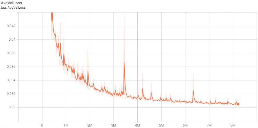
Tensorboard is excellent for monitoring the progress of training and viewing a few sample results from each epoch. It’s well worth the time to integrate and run it. Example Tensorboard validation loss graph:
To run the training on multiple GPUs and nodes, I initially tried using the HuggingFace accelerate library and also vanilla PyTorch DDP, but found that both methods were much slower than Microsoft DeepSpeed and much more finnicky to use.
Microsoft DeepSpeed was a huge help especially for multi-GPU and multi-node training. It simplifies PyTorch code in a similar way to PyTorch Lightning, but adds a ton of value. I can launch training with one command. Its launcher script is very robust and CTRL+C does what you expect to stop training quickly. It has a nice API for Tensorboard, gradient accumulation, learning rate scheduling, ADAM optimizer, robust fast FP16 training, checkpointing and resuming. It seems to do a good job with IPC because I haven’t noticed any bottlenecks related to node-to-node communication. There are also some features for training much larger models with ZeRO optimization, which I probably will never use.
Logging is more complicated when using DeepSpeed. After fiddling around a bunch, I ended up with these helper functions:
import deepspeed
from deepspeed import comm
from deepspeed import log_dist

def log_0(msg):
    log_dist(msg, ranks=[0])

def log_all(msg):
    log_dist(msg, ranks=[-1])

def is_main_process():
    return comm.get_rank() == 0
The log_0 function only logs from the rank=0 (primary) script process. And log_all will log from all the instances. Other logging methods like print() or the logging subsystem will end up being jumbled or not printing. The is_main_process function allows the code to do some calculations only on the primary machine’s main process. Note that DeepSpeed uses multiple processes per machine so it can get complicated unless you work within the framework.
I started integrating Microsoft NNI, which allows you to automate architecture search for neural networks, but haven’t had a chance to experiment with it yet. It seems like it might be useful for finding the best architecture for super-resolution, or NeRF, or some other projects I’m interested in.
I experimented with Torch Dynamo and found that it was a quick performance win. It’s a JIT compiler for PyTorch that speeds up the training loop. I found that it wasn’t providing any benefit to optimize the model itself, but I found that wrapping the model forward pass and loss calculation in a function and optimizing those together did improve performance. This was as easy as adding one line of code: forward_and_loss = dynamo.optimize("eager")(forward_and_loss) so seems worth trying. There is supposed to be a better “inductor” optimizer but it seems to be broken right now.
I found these tweaks to speed up training:
# Enable cuDNN benchmarking to improve online performance
torch.backends.cudnn.benchmark = True

# Disable profiling to speed up training
torch.autograd.profiler.emit_nvtx(False)
torch.autograd.profiler.profile(False)
For data loading I’m using the Nvidia DALI library, which is a fast framework for loading PNG and JPG images. The JPG image loading is much faster than the PNG image loading, but it does not matter too much (see next section for more info).
I think I saw that my training scripts had some issues when the batch size is not a power of two, so to keep things simple I’d recommend using a number like 32 or 64 for batch size. The difference in training speed between a batch size of 16 and 32 is actually not that much, so just rounding to the nearest power of two that will fit in VRAM is fine and any bugs can be ignored. It might be a bug in DeepSpeed also not sure to be honest.
Datasets and Data Loading⌗
Initially I was planning to use a huge amount of data for training, but I found pretty quickly that about 20K 512x512 images are sufficient for upsampling models. Probably not even that many are needed. There are some high quality datasets already available that are commonly used in super-resolution research such as DIV2K and Flickr2K used by the VapSR researchers. I put all the datasets up on Google Drive and where I found them: https://drive.google.com/drive/folders/1kILRdaxD2o273E2NnrXzhaLbQCXDxz9l The code for this project also includes scripts for working with ImageNet data, and ripping datasets from 4K Blu-Ray discs, but it turned out to not be necessary.
The trick seems to be to watch the training loss and validation loss charts. If the validation loss is getting worse, it means the data is overfitting to the training set, so probably more data is required.
Once I started actually training the models I found that having a “right sized” dataset that can be trained repeatedly is more convenient than a huge dataset. Epochs that take 20 seconds to complete are really convenient for testing and debugging, and the performance might even be better than training on a huge dataset, though I haven’t tested that. A knowledgeable friend said that it’s probably helpful to have a dataset that is smaller so the model can learn more features of the data.
Normally people use images that are different sizes and perform random crops on each image, but since I initially wanted to work with enormous datasets, I built a framework for performing random 512x512 crops so that the DALI data loader has consistently-sized images to load. This does leave out some parts of the training images, but that can always be counter-acted by adding more data. All the tooling I wrote allows for full CPU parallelism and some quick shortcuts to validate the files, processing the datasets extremely quickly. So, unintentionally I solved some large data loading challenges that I did not need to solve, but it’s nice to have the framework now since it might be useful one day.
I found that JPEG images load much faster in DALI than PNG images using the GPU, though JPEGs are lossy and for my super-resolution project I did not want to have to deal with image artifacts, so I ended up using PNG images. DALI still does a much better job than vanilla PyTorch or NumPy at loading images fast, after implementing both ways and profiling them.
I also tried JPEG-2000 (also supported by DALI) and WebP, but found that both options are much too slow in practice.
I tried varying the colorspace of the data as well, trying RGB (typical), YUV, and OKLAB. The idea was to make the input data easier for the model to work on. OKLAB, for example, was designed for use in image resamplers since averaging pixels together does not cause the brightness of the pixels to change incorrectly. However, I found that converting the data to OKLAB or YUV inside the network, and then converting back to RGB at the end caused a significant loss in quality. So, I ended up sticking with RGB. My theory is that if the data itself was in OKLAB or YUV format then there would be some advantage. However since I’m trying to work towards real-time video upsampling, adding extra image processing operations is probably a bad idea for performance reasons. Also, video is in YUV format already, so no conversion will be needed - Instead the model would be trained on images in YUV colorspace.
Since I’m not trying to win benchmarks, I’m using 1% of the dataset as a validation set to monitor the training progress, so for 20K images that works out to about 200 images. Usually researchers keep these separate to maximize their benchmark scores, but it’s not useful in practice, and just selecting training/validation images randomly from the same set is fine. I didn’t mix in any test images into the training set for fair comparison however. I wouldn’t use a much smaller validation set than this, since the loss seems much noisier than on the training set. If I had more time I’d probably try adding more training data and use more like 500 images for validation just to eliminate the noise a bit more.
Data Augmentation⌗
The validation images need to be the same for each epoch so that I can directly compare the loss for each epoch. However for the training data I’m applying data augmentation in the DALI data loader using random crops, random horizontal flips, and random 90 degree rotations. These are all operations that do not mix data between pixels.
Through progressively adding more augmentations to the data, I’ve found that the network learns better the more that are applied. When I first added random horizontal flips I noticed improvements in quality early on, and later I quantified that adding random rotations added 0.15 dB PSNR, which is a huge jump in quality.
I tried using smaller 128x128 crops instead of 256x256 crops and using a 4x larger batch size, with the intuition that it might lead to better generalization. The results were not as good, about 0.03 dB worse.
Choice of Downsampling Function⌗
There are three major choices for downsampling images as input to this model:
- Bicubic downsampling.
- Gaussian downsampling.
- Jointly learned downsampling.
Of all the traditional image processing kernels for downsampling-then-upsampling, bicubic performs the best in my own prior evaluation. I implemented and benchmarked Lanczos, Mitchell, Hermite, Cubic Spline, Sinc, and other cubic kernels at Anduril using Halide-Lang and found that the best option depends on the operation, but for 2x or 4x downsampling followed by 2x or 4x upsampling, bicubic preserved the most information in the original image. Also I’m seeing all the super-resolution papers use this function.
Gaussian downsampling I did not test actually, but I’ve used that for producing image pyramids for frame-to-frame alignment for video stabilization. Since it tends to produce sharper images than bicubic, the model would need to be trained on this type of downsampler to be able to work with it. In practice, it might work better overall than bicubic, but I haven’t trained my model using this type of data. Mainly because it was outside the scope of my project, and it required more work to implement in the data loader. However, I do recall one paper that compared bicubic and Gaussian downsampling and found that Gaussian downsampling performed very slightly better when used with a learned upsampler, so probably it’s a good idea.
Jointly learned downsampling is the best option by far. I didn’t implement this because it’s a lot more work, but I’ve seen 3 different papers that independently reproduced a 3dB improvement in upsampler performance over bicubic downsampling, so it’s almost certainly worth doing for a practical application. These results have given me the intuition that it’s well worth doing at least some work on the encoder side as well.
Normalization and Layout⌗
The input and output images are fairly convenient to be processed by CPU in 8-bit RGB or YUV format, so it seems fine to use a different layout for the network. For training, I used the NCHW layout that seems to be preferred by all GPU codebases for performance. I’m aware that CPU inference tends to prefer NHWC layout for cache locality, which is what I’m familiar with for image processing kernels. I decided not to do any layout changes inside the network, and rely on the code running inference to do layout conversion.
For the uninitiated, NCHW means N=batch of images, C=color channel, H=height, W=width, and each color channel is stored on separate planes. We also call this multi-planar color in image processing terms.
However, I think that normalization has some advantages when done inside the model so that it can be done with FP16 precision using tensor cores. So I took the somewhat unusual step to do normalization from 0..255 uint8 RGB input to -1..1 FP16 RGB input inside the network, and to convert back to 0..255 uint8 RGB output at the end. For example when the network is run in OpenVINO, the normalization preprocessing is done on CPU which does not support FP16. This means that the network does slightly different things during training and during inference, but I think it’s a reasonable tradeoff. This simplifies the data loader since it does not need to care about normalization stuff. The main wart is that it does make the loss function more complicated since it needs to normalize the target images to compare to the output of the model during training. This does not affect training speed, however.
Another interesting advantage is that moving data to the GPU from the CPU is 2x more efficient if normalization is done in-network, so it makes a lot of sense to me. It uses half the bandwidth because the data it’s moving is half the size. Similarly, if I was using multi-planar YUV 4:2:0 input, where the UV channels are half the size of the Y channel, I would also want to do any colorspace conversion in the network.
My understanding is that data within the model should generally be normalized and range from -1 to 1, so that’s how the RGB channels are normalized going into the network. As far as I know, using 0..1 is just as good for training but I haven’t checked if it has any effect. Personally I think the wacky ImageNet normalization factors should be considered harmful, since they add unnecessary complexity. I suspect they do not change the performance of the model.
One place where normalization does matter is in calculating PSNR, SSIM, and LPIPS scores for the test set. This is done in evaluate.py in my project. It’s important to carefully set up the data normalization and the calculations to be compatible. For example, PSNR and SSIM are usually calculated on data normalized from 0..1 instead of -1..1, and you need to parameterize the functions appropriately for the data range. LPIPS requires values normalized to -1..1.
Training⌗
My general training strategy has been to keep things simple and use the DeepSpeed defaults, which seem to work pretty well. I use an early-stopping strategy where the training continues until the validation fails to improve for 200 epochs. This seems to be sufficient to thoroughly train the network.
Based on some feedback from peers, I tried training using FP32 and FP16. I found that FP32 did improve PSNR of the model by 0.01 dB on the test set, but this is not significant enough to warrant the huge increase in training time, so FP16 seems like a huge win.
I tried L1 loss as used in VapSR, and found that it indeed worked the best. MSE loss led to worse PSNR on the test set, about 0.3 dB worse. I also tried LPIPS (human perception based) loss and found that it was not effective.
Thanks to all the hardware and optimizations discussed above, I’m able to fully train a super-resolution network in about 6 hours.
The code is all fairly well documented here: https://github.com/catid/upsampling - The README describes how to reproduce my results.
Inference⌗
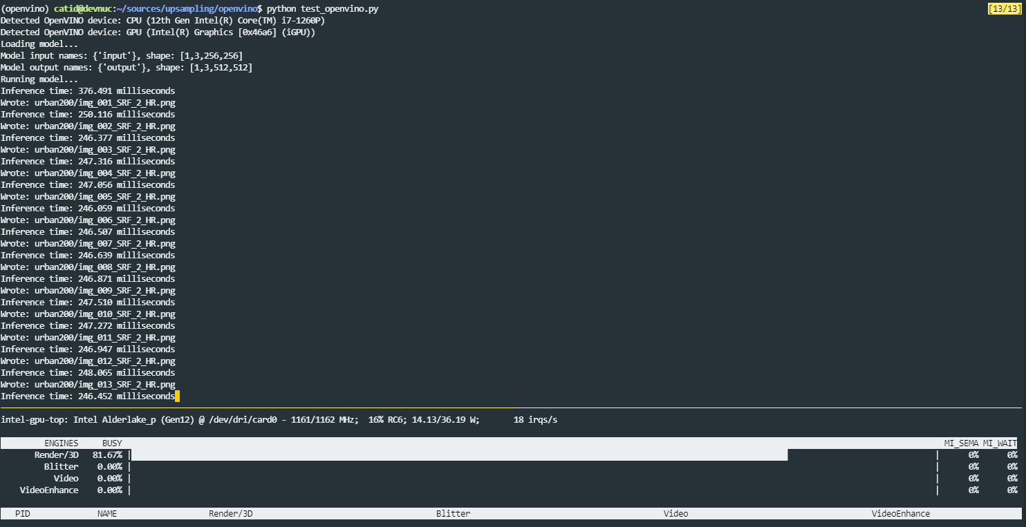
Inference using PyTorch is fairly straight-forward and there’s an example in the evaluate.py script, but I’m more interested in getting the best performance possible out of the Intel GPU just using the lower-level Intel APIs. So in addition, I learned how to set up and use OpenVINO. I wrote a bunch of documentation for this in the openvino directory here: https://github.com/catid/upsampling/tree/master/openvino
Results⌗
The results of the model I trained are excellent. On the Urban100 dataset, the model achieves a PSNR of 30.53 dB, which is 5.66 dB better than bicubic upsampling. This is a very significant improvement in quality, almost 4x better, and close in quality to the original images. This is not the best result ever achieved, but it is better than the VapSR paper result. It’s also a fairly small network designed to run fast, so it’s not really optimized for the best possible quality.
The results for OpenVINO inference on Intel GPU are less spectacular. It runs at about 2x the speed of the CPU, but far from video frame-rates. It takes about 250 milliseconds to upsample a 256x256 input image to 512x512. So, it seems like it would run at about 1 FPS on HD video. Optimizing the model to run at 60 FPS is a future project, which will probably involve giving up a lot of image quality and using 8-bit quantization.
I’m not sure if I’ll be using this specific model design for my next project working towards a video codec. The cutting-edge paper I shared by Zhang et al seems to be a better starting point, though some ideas from this work could be useful.
But, it’s a good start and I learned a lot from this project. I can confidently say now that I know enough about machine learning to be dangerous.